Usage

This section describes the general usage of the software. Follow the next subsections to calculate a treatment, generate a report and send it to a R&V system with Kali MC.

Applicator

Choose between the available applicator diameters (3, 4, 5, 6, 7, 8, 9, 10 and 12 cm) and bevel endings (0º, 15º, 30º and 45º).

Prescription

Enter the prescribed dose in cGy and the desired depth in cm (depth of the 90% isodose).

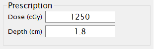
Energy selection

Choose the desired energy comparing its R₉₀ with the prescribed treatment depth.

Note

If rescaling factors are enabled in local_conf.py, the associated factors will show next to the R₉₀ values.

MU calculation

Once the diameter, bevel of the applicator, and the desired energy are selected, it is necessary to enter the current atmospheric pressure in hPa. This is required because the monitor system of the linac does not perform pressure correction, and undesirable output deviations can occur if this correction is not made.

For that purpose, the atmospheric pressure at the time of the equipment calibration (P_ref ) must be recorded.

Note

You can modify this parameter customizing the configuration file, local_conf.py (see the Configuration file section).

The following expression is used for calculating Monitor Units:

\[UM = round(\frac{D * P_{now} * f_{resc}} {cGy/UM * (iso_{presc} / 100) * P_{ref}})\]

where:

D: Prescribed Dose in cGy
P_now: Current atmospheric pressure (hPa)
f_resc: Rescaling factor, if activated, otherwise f_resc=1
cGy/UM: Output factor at z_max for the current applicator and energy combination in cGy per MU.
iso_presc: Prescription relative isodose, non-editable, 90% isodose.
P_ref: Atmospheric pressure (hPa) at calibration time.

If a second calculation has been performed (hand calculation or with a different software), the result can be entered, and a deviation will be calculated as a quotient between the two values, expressed in percentage.

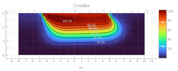
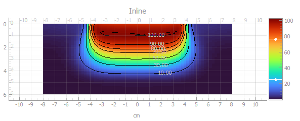
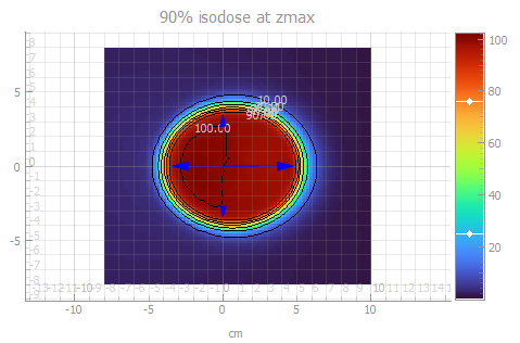
Dose distributions

The software shows dose planes with relative isodose levels in the crossline and inline directions, as well as in a coronal plane at the depth of z_max of the selected energy/applicator. When inclined applicators are selected, the major axis is aligned along the crossline direction.

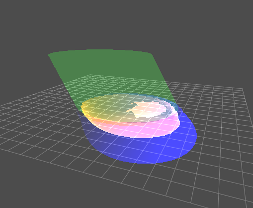
Additionally, there is a 3D view of the applicator and the isodoses at 20%, 90%, and 105%.

All dose distributions are normalized to the absorbed dose at z_max in the clinical axis.

Crossline
Inline
Coronal at z_max
3D

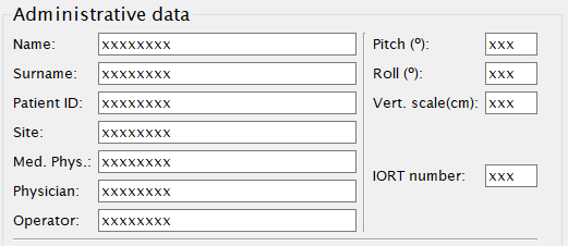
Report generation

A PDF report can be generated; for this purpose, some administrative data must be provided:

Press the Generate report button:

Use the save file dialog to choose the destination path of the pdf file.

Note

The default path for saving reports can be customized in the local_conf.py file, see the Configuration file section.

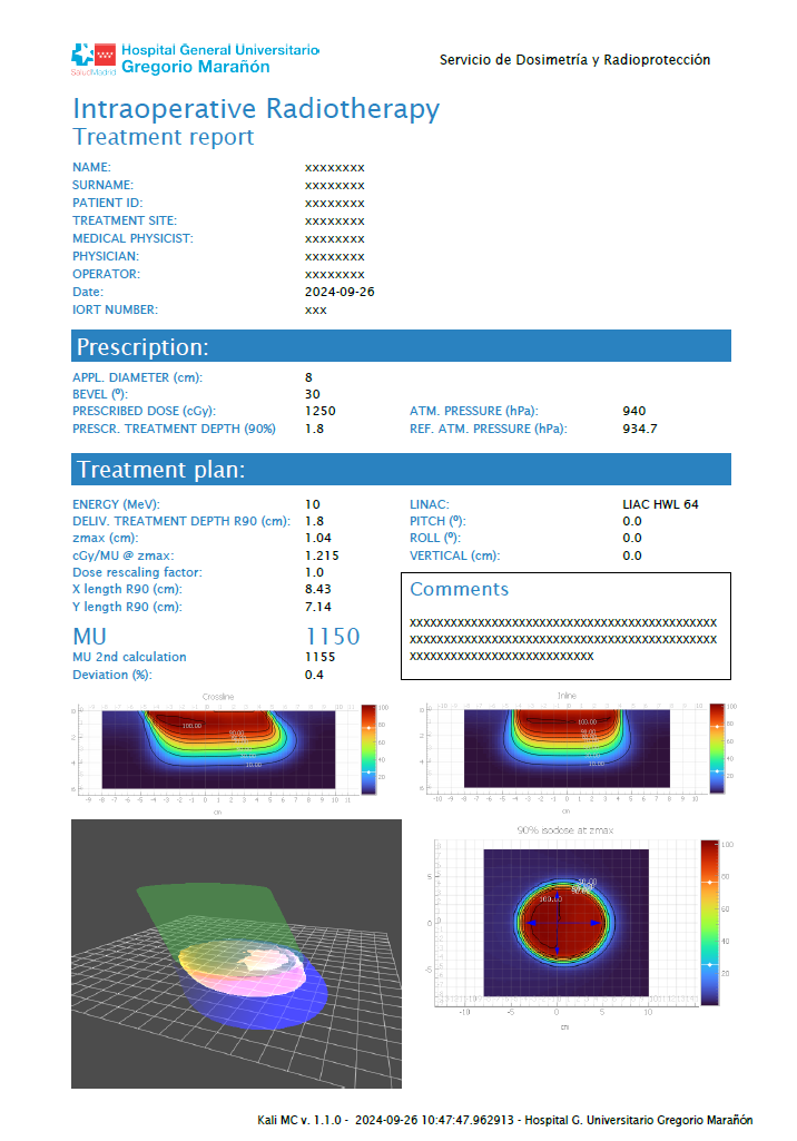
A report will be generated with the treatment data:

Note

The institution logo and department name can be customized in the local_conf.py file, see the Configuration file section.

Send plan to R&V systems

The prescription and treatment parameters can be sent to a Record and Verify system as a DICOM RTPlan object. The following items need to be configured in the local_conf.py file:

destination_server
destination_AETitle
destination_port

If exporting to Elekta Mosaiq, the machine name in Mosaiq must match the exported name. You can modify this using the machine parameter:

machine

Additionally, Mosaiq attempts to match tolerance tables when importing a plan. While this is not strictly necessary, it can simplify the import process. You can modify tolerances with the following parameters:

tol_table_ID
tol_table_label

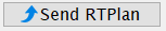
Once the administrative data is filled and the server is configured in the local_conf.py file, the exportation is done by pressing the Send RTPlan button:

Note

The applicator names are sent as C10B0, C3B45… In order to map them in Mosaiq, they have to be defined in the machine characterization.